9.6. ROC(Receiver Operating Characteristic)について
医学と統計(52)投稿からから。
統計解析環境「R」を使ったROC曲線などの分析事例を紹介します。
ここでは心筋梗塞(Inf.)と狭心症(Ang.)の有(1)無(0)における血清CPK(Creatine phosphokinase )の仮想データを用いる事にします。
「R」コマンドの記述
library(Epi)
CPK<- c( 452, 462, 456, 456, 458, 421, 391, 394, 384, 427, 298, 295, 257, 244, 262,
254, 226, 203, 219, 236, 174, 178, 194, 197, 143, 159, 136, 126, 116, 105,
104, 87, 96, 118, 60, 66, 68, 52, 15, 36, 7, 38, 27, 7, 7, 4 )
Inf.<- c( 1, 1, 1, 1, 1, 1, 1, 1, 1, 1, 1, 1, 1, 1, 1, 0, 1, 1, 1, 0, 1, 1, 1, 0, 1, 1, 1, 1, 1, 1,
1, 1, 0, 0, 1, 1, 0, 0, 1, 0, 0, 0, 0, 0, 0, 0 )
Ang.<- c( 1, 1, 1, 1, 1, 1, 1, 1, 1, 1, 1, 1, 1, 0, 1, 1, 1, 1, 0, 1, 1, 1, 1, 1, 1, 1, 1, 1, 0, 0,
1, 1, 1, 1, 1, 1, 0, 0, 1, 0, 0, 0, 0, 0, 0, 0 )
ROC(CPK, Inf., plot="ROC", PV=T, MX=T, MI=T, AUC=T)
上記のデータを表計算ソフト「MS-Excel」 に入力しておき、下記コマンドを実行する方が便利でしょう (入力済みデータはここから)
library(Epi)
dat<- read.delim("clipboard", header=T)
x<- dat$CPK
y<- dat$Inf.
z<- dat$Ang.
ROC(x, y, plot="ROC", PV=T, MX=T, MI=T, AUC=T)
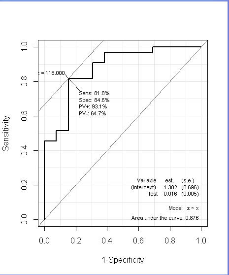
ROC(x, z, plot="ROC", PV=T, MX=T, MI=T, AUC=T)
*** >br>
Arguments (引数)
PV: Should sensitivity, specificity and predictive values at the optimal cutpoint be given on the ROC plot?
MX: Should the “optimal cutpoint” (i.e. where sens+spec is maximal) be indicated on the ROC curve?
MI : Should model summary from the logistic regression model be printed in the plot?
***
出力結果:
図1:心筋梗塞(Inf.)のROC
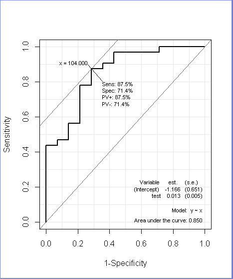
図2:狭心症(Ang.)のROC
重ね書きしたい時は次の様にすれば良いでしょう。
ROC(x, y, plot="ROC", PV=F, MX=F, MI=F, AUC=F)
par(new=T,col=2)
ROC(x, z, plot="ROC", PV=F, MX=F, MI=F, AUC=F)
Logistic model への当てはめは次により行うことが出来ます。
library(Epi)
mod <- glm ( y ~ x , data=dat , family=binomial )
y.hat <- fitted ( mod , type = "response" )
ROC ( y.hat , y , PV=F , MX=F , MI = F , cuts = 0.5 , plot="ROC" )
classtab <- function(yy , pred, cutoff){
tmp.y <- factor ( yy , levels=c ( 0 , 1 ) , labels = c ( "True 0" , "True 1" ) )
pred.y <- factor ( as.numeric ( pred > cutoff ) , levels = c ( 0 , 1 ) ,
labels = c ( "Predicted + tab <- table ( pred.y , tmp.y , deparse.level = 0 )
class(tab) <- "classtab"
return(tab=tab)
}
print.classtab <- function ( obj ) { noquote ( print ( obj [1: 2 , 1: 2 ] ) )
cat ( "\n" )
cat ( "Sensitivity = ", round ( obj [ 2 , 2 ] / sum ( obj [ , 2 ] ) , 3 ) , "\n")
cat ( "Specificity = ", round ( obj [ 1 , 1 ] / sum ( obj [ , 1 ] ) , 3 ) , "\n")
}
ctab <- classtab ( y , fitted(mod , type = "response" ) , 0.5 )
ctab
出力結果
| ... | True(0) | True(1) |
| Predicted(0) | 9 | 3 |
| Predicted(1) | 5 | 29 |
Sensitivity = 0.906
Specificity = 0.643
上記の出力結果は Logistic 回帰モデルで Cutoff = 0.5 とした場合です。
ところで、
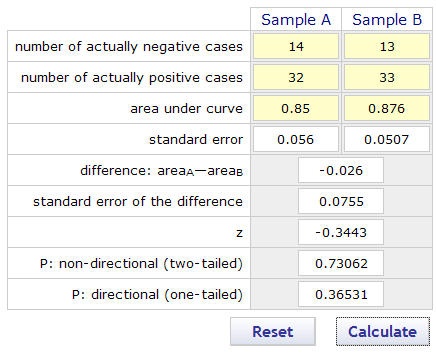
心筋梗塞(Inf.)と狭心症(Ang.)の2つのAUCの比較は次により行うことが出来ます。
Web オンラインソフト(下記URL)を使って見ましょう。
参照URL
出力結果
Significance of the Difference between the Areas under Two Independent ROC Curves
「R」では、
library( pROC ) が用意されていますので、次により行います。
参照先URL
library のインストール( pROC , plyr )をしておきます。
そして、実行は次の通りです。
library(pROC)
roc.Inf <- roc ( CPK ~ Inf., data = dat )
roc.Ang <- roc( CPK ~ Ang.., data=dat )
roc.Inf
roc.Ang
roc.test ( roc1 = roc.Inf , roc2 = roc.Ang , method = "delong" )
# Bootstrap 法
roc.test ( roc1 = roc.Inf, roc2 = roc.Ang, method = "bootstrap", boot.n = 1000 )
*** 詳しくは下記URLの「pROC.pdf」を参考にして下さい。 参照先URL ***
出力結果:
DeLong's test for two ROC curves
data: roc.Inf and roc.Ang
D = -0.3029, df = 89.475, p-value = 0.7626
alternative hypothesis: true difference in AUC is not equal to 0
sample estimates:
AUC of roc1 AUC of roc2
0.8504464 0.8764569
戻る 次へ 目次へ TOPへ